LLM Inference Optimization: 2026 Update - MTP Deep Dive
Estimated Reading Time: 8 minutes
TLDR
In 2023, speculative decoding was about “The Big Model and its Small Friend.” By 2026, the paradigm has shifted toward Architectural Integration. Multi-Token Prediction (MTP) and its distilled counterpart (MTP-D) have replaced external draft models by embedding “future-thinking” heads directly into the main model’s trunk. This article explores the mechanics of validation, the “mini-prefill” paradox, and why alignment—not just accuracy—is the key to 2x+ throughput.
1. The Foundation: Standard Speculative Decoding & The Memory Wall
To understand why MTP is a game-changer, we must first look at why standard autoregressive decoding is slow. LLM inference is traditionally memory-bandwidth bound: the GPU spends 99% of its time moving weights from VRAM to compute cores and only 1% doing math.
The Paradox: Why is “More Work” Faster?
It seems counterintuitive that doing more computational work—running a large model on a draft of $K$ tokens—is faster than running it on just one. The answer lies in the Arithmetic Intensity of the GPU. Because loading the model weights from memory is the primary bottleneck, the “time-cost” of a forward pass is nearly identical whether you process 1 token or 20 tokens.
By verifying $K$ tokens in parallel, we aren’t adding more time; we are simply utilizing the idle compute cores that were already waiting for the weights to arrive.
The “Mini-Prefill” Analog
Speculative decoding utilizes this hardware reality to perform a mini-prefill. This technique, pioneered in early works like those by Leviathan et al. 1 and Xia et al. 2, effectively trades idle compute for a reduction in memory loading cycles:
- The Draft: A fast mechanism (like a small model) guesses $K$ tokens.
- The Parallel Validation: The large model takes all $K$ tokens at once. It performs the verification in a single forward pass—essentially getting $K$ tokens for the price of one “memory-loading” trip.
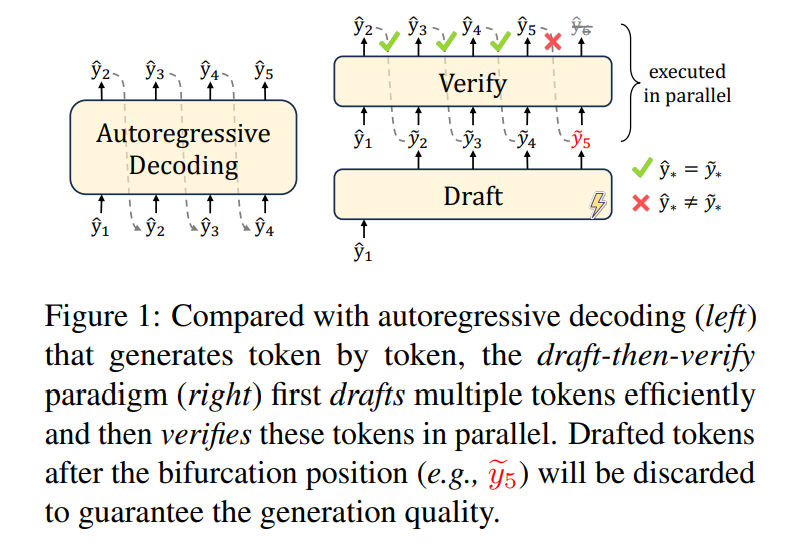
Figure 1: Traditional Speculative Decoding architecture (Draft-Target paradigm)
2. Multi-Token Prediction (MTP): The Sidecar Architecture
MTP solves the “Alignment Problem.” In early implementations, the draft model often “hallucinated” a different path than the target model because they were different architectures. MTP solves this by using a Shared Trunk approach popularized by the DeepSeek-V3 3 and Qwen3 4 series.
The Anatomy of an MTP Model
- The Shared Trunk: All layers of the main model (the “brain”) are used to process the context.
- MTP Modules: These are lightweight Transformer layers attached after the final layer of the trunk, typically predicting 2-4 tokens ahead as detailed in Gloeckle et al. 5.
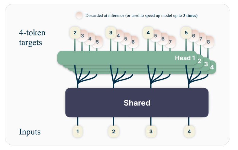
Figure 2: MTP Shared Trunk Architecture with integrated prediction heads
The Inference Flow (Same for MTP & MTP-D)
From an execution standpoint, MTP and MTP-D are identical. The “D” does not change the inference path; it only changes how the weights were learned.
- Trunk Pass: The main model processes token $t$ through its full depth to get hidden state $h_t$.
- Branching:
- Main Head: Predicts $t+1$.
- MTP Head 1: Takes $h_t$ + embedding of $t+1$ to predict $t+2$.
- MTP Head 2: Takes the output of Head 1 to predict $t+3$.
- One-Shot Validation: The main model validates $t+2$ and $t+3$ in a parallel pass.
3. Beyond Accuracy: Why MTP-D Wins
While the inference path is shared, the Training Path is where MTP-D (Self-Distilled MTP) diverges to become the true game-changer of 2026.
Alignment vs. Prediction
The problem with standard MTP is that it tries to predict the “ground truth” labels of the dataset. However, in inference, we don’t care if the MTP head is accurate to the dataset; we only care if it is accurate to the main model.
MTP-D shifts the objective from “predicting the next word” to “predicting the main model’s mind.” This behavioral alignment, explored in recent research 6, is what pushes acceptance rates from a shaky 60% to a reliable 90%+.
The Two-Stage Training Process
Stage 1: Joint MTP Pre-training
The model is first optimized for both Next-Token Prediction (NTP) and Multi-Token Prediction (MTP). This stage is often included in modern pre-training surveys 7 as a way to improve representation learning.
\[L_{Joint} = L_{NTP}(t+1) + \lambda \sum_{i=1}^{K} L_{CE}(P_{head\_i}, \text{label}_{t+i+1})\]Stage 2: MTP-D (Self-Distillation)
Once the trunk is stable, we move to a dedicated Self-Distillation step. The Trunk is typically frozen (Stop-Gradient), and we optimize only the MTP heads to mimic the Trunk’s internal logits.
\[L_{MTP-D}^{(i)} = L_{CE}(P_{head\_i}, \text{label}) + \beta \cdot D_{KL}(sg(P_{target}) \parallel P_{head\_i})\]- The Soft Target: The $D_{KL}$ term ensures the head’s probability distribution matches the main model’s “beliefs.” Even if the main model makes a non-obvious choice, the MTP-D head anticipates it, ensuring the speculative chain doesn’t break.
4. Optimization Trade-offs: The $K$ Factor
The choice of $K$ (look-ahead window) balances GPU utilization against error compounding.
| Strategy | $K$ Value | Industry Standard Use Case |
|---|---|---|
| Conservative | $K=1-2$ | Highly creative or complex reasoning tasks. |
| Balanced | $K=3-5$ | General Assistant / Chat (The “Sweet Spot”). |
| Aggressive | $K=6-10$ | Structured Data (JSON, Code, or repetitive logs). |
5. Conclusion: The 2026 Outlook
We have reached the end of the “Dual Model” era. Today’s state-of-the-art inference engines don’t look for a “fast small model” to pair with a “smart big model.” Instead, they utilize MTP-D to build a single, cohesive engine that naturally thinks 3-4 steps ahead. By aligning the “future-thinking” heads with the main model’s internal logic during the training path, we can effectively double throughput in the inference path without sacrificing accuracy.
References
-
Leviathan, Yaniv, et al. “Fast inference from transformers via speculative decoding.” (2023). ↩
-
Xia, Heming, et al. “Speculative Decoding: Exploiting Speculative Execution for Accelerating Seq2seq Generation.” (2022). ↩
-
DeepSeek-AI. “DeepSeek-V3 Technical Report.” (2025). ↩
-
Alibaba Group. “Alibaba Open-Sources Qwen3.5 with Native MTP Heads.” (2026). ↩
-
Gloeckle, Fabian, et al. “Better & Faster Large Language Models via Multi-token Prediction.” (2024). ↩
-
Zhao et al. “Self-Distilled Multi-Token Prediction for Efficient Inference.” (2026). ↩
-
Xu, Jiawei, et al. “A Comprehensive Survey on Large Language Models: From Pre-training to Autonomous Agents.” (2025). ↩